Appendix
8.1 SPDE and Triangulation
In order to fit LGM type of models with a spatial component INLA uses SPDE (Stochastic Partial Differential Equations) approach. Suppose that is it given have a continuous Gaussian random process (a general continuous surface), what SPDE does is to approximate the continuous process by a discrete Gaussian process using a triangulation of the region of the study. Let assume to have a set of points defined by a CRS system (Latitude and Longitude, Easthings and Northings), and let assume that the object of the analysis is to estimate a spatially continuous process. Instead of exploiting this property as a whole, it is estimated the process only at the vertices of this triangulation. This requires to put a Triangulation of the region of the study on top the the process and the software will predict the value of the process at its vertices, then it interpolates the rest of the points obtaining a “scattered” surface.
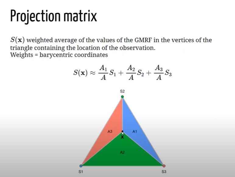
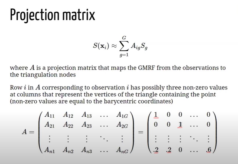
Imagine to have a point a location X laying inside a triangle whose vertices are \(S_1, S_2 and S_3\). SPDE operates by setting the values of the process at location x equal to the value of the process at their vertices with some weights, and the weights are given by the Baricentric coordinates (BC). BC are proportional to the area at the point and the vertices. Let assume to have a piece of Triangulation \(\boldsymbol{A}\) and let assume that the goal is to compute the value at location X. X, as in formula above \(\boldsymbol{A}\), would be equal to \(S_1\), multiplied by the area \(A_1\) dived by the whole triangle area (\(\boldsymbol{A}\)) + \(S_2\) multiplied by the area \(A_2\) divided by \(\boldsymbol{A}\) + \(S_3\), multiplied by the area \(A_3\) dived by (\(\boldsymbol{A}\). This would be the value of the process at location X given the triangulations (number of vertices). SPDE is actually approximating the value of the process using a weighted average of the value of the process at the triangle vertices which ir proportional to the area of the below triangle. In order to do this within INLA 4 it is needed also a Projection Matrix , figure 8.4. The Projection matrix maps the continuous GRMF (when it is assumed a GP) from the observation to the triangulation. It essentially assigns the height of the triangle for each vertex of the Triangulation to the process. Matrix \(\mathcal{A}\), whose dimensions are \(\mathcal{A_{ng}}\). It has \(n\) rows a \(g\) columns, where \(n\) is the number of observations and \(g\) is the number of vertices of the triangulation. Each row has possibly three non-0 values, right matrix in figure 8.4, and the columns represent the vertices of the triangles that contains the point. Assume to have an observation that coincides with a vertex \(S_1\) of the triangle in 8.3, since the point is on top of the vertex (not inside), there are no weights (\(A_1 = \mathcal{A}\)) and 1 would be the value at \(A_{(1,1)}\) and 0 would be the rest f the values in the row. Now let assume to have an observation coinciding with \(S_3\) (vertex in position 3), then the result for \(A_{(2,3)}\) would be 1 and the rest 0. Indeed when tha value is X that lies within one of the triangles all the elements of the rows will be 0, but three elements in the row corresponding of the p osition of the vertices \(1 = .2, 2 = .2 and g = .6\), as a result X will be weighted down for the areas.
8.2 Laplace Approximation
Michela Blangiardo Marta; Cameletti (2015) offers an INLA focused intuiton on how the Laplace approximation works for integrals. Let assume that the interest is to compute the follwing integral, assuming the notation followed throughout the analysis:
\[ \int \pi(x) \mathrm{d} x=\int \exp (\log f(x)) \mathrm{d} x \] Where \(X\) is a random variable for which it is specified a distribution function \(\pi\). Then by the Taylor series expansions (Fosso-Tande 2008) it is possible to represent the \(\log \pi(x)\) evaluated in an exact point \(x = x_0\), so that:
\[\begin{equation} \log \pi(x) \approx \log \pi\left(x_{0}\right)+\left.\left(x-x_{0}\right) \frac{\partial \log \pi(x)}{\partial x}\right|_{x=x_{0}}+\left.\frac{\left(x-x_{0}\right)^{2}}{2} \frac{\partial^{2} \log \pi(x)}{\partial x^{2}}\right|_{x=x_{0}} \tag{8.1} \end{equation}\]
Then if it is assumed that \(x_0\) is set equal to the mode \(x_*\) of the distribution (the highest point), for which \(x_{*}=\operatorname{argmax}_{x} \log \pi(x)\), then the first order derivative with respect to \(x\) is 0, i.e. \(\left.\frac{\partial \log f(x)}{\partial x}\right|_{x=x_{*}}=0\). That comes natural since once the function reaches its peak, i.e. the max then the derivative in that point is 0. Then by leaving out the first derivative element in eq. (8.1) it is obtained:
\[ \log \pi(x) \approx \log \pi\left(x_{*}\right)+\left.\frac{\left(x-x_{*}\right)^{2}}{2} \frac{\partial^{2} \log \pi(x)}{\partial x^{2}}\right|_{x=x_{*}} \]
Then by integrating what remained, exponantiating and taking out non integrable terms,
\[\begin{equation} \int \pi(x) \mathrm{d} x \approx \exp \left(\log \pi\left(x_{*}\right)\right) \int \exp \left(\left.\frac{\left(x-x_{*}\right)^{2}}{2} \frac{\partial^{2} \log \pi(x)}{\partial x^{2}}\right|_{x=x_{*}}\right) \mathrm{d} x \tag{8.2} \end{equation}\]
At this point it might be already intuited the expression (8.2) is actually the density of a Normal. As a matter of fact, by imposing \(\sigma^{2}_{*}=-1 /\left.\frac{\partial^{2} \log f(x)}{\partial x^{2}}\right|_{x=x_{*}}\), then expression (8.2) can be rewritten as:
\[\begin{equation} \int \pi(x) \mathrm{d} x \approx \exp \left(\log \pi\left(x_{*}\right)\right) \int \exp \left(-\frac{\left(x-x_{*}\right)^{2}}{2 \sigma^{2}_{*}}\right) \mathrm{d} x \tag{8.3} \end{equation}\]
Furthermore the integrand is the Kernel of the Normal distribution having mean equal to the mode \(x_*\) and variance specified as \(\sigma^{2}_{*}\). By computing the finite integral of (8.3) on the closed neighbor \([ \alpha, \beta]\) the approximation becomes:
\[ \int_{\alpha}^{\beta} f(x) \mathrm{d} x \approx \pi\left(x_{*}\right) \sqrt{2 \pi \sigma^{2^{*}}}(\Phi(\beta)-\Phi(\alpha)) \] where \(\Phi(\cdot)\) is the cumulative distribution function corresponding value of the Normal disttribution in eq. (8.3).
For example consider the Chi-squared \(\chi^{2}\) density function (since it is easily differentiable and Gamma \(\Gamma\) term in denominator is constant). The following quantities of interest are the \(\log \pi(x)\), then the \(\frac{\partial \log \pi(x)}{\partial x}\), which has to be set equal to 0 to find the integrating point, and finally \(\log \pi(x)\) \(\frac{\partial^2 \log \pi(x)}{\partial x^2}\). The \(\chi^{2}\) pdf, whose support is \(x \in \mathbb{R}^{+}\) and whose degrees of freedom are \(k\):
\[ \chi^{2}(x,k)=\frac{x^{(k / 2-1)} e^{-x / 2}}{2^{k / 2} \,\, \Gamma\left(\frac{k}{2}\right)}, x \geq 0 \]
for which are computed:
\[ \log f(x)=(k / 2-1) \log x-x / 2 \] Ths single variable Score Function and the \(x_{*}=\operatorname{argmax}_{x} \log \pi(x)\),
\[\begin{equation} \begin{aligned} &\frac{\partial \log \pi(x)}{\partial x}= \frac{(k/2 -1)}{x} - \frac{1}{2} =0 \quad \text {solving for 0 }\\ &(k/2-1) = x/2\quad \text {moving addends}\\ &x_* = (k-2) \end{aligned} \end{equation}\]
And the Fisher Information in the \(x_*\) (for which it is known \(\sigma^{2}_*=-1 / f^{\prime \prime}(x)\))
\[\begin{equation} \begin{split} &\frac{\partial^2 \log \pi(x)}{\partial x^2}=-\frac{(k / 2-1) }{x^{2}} \quad \text {substituting} \,\,x_* \\ &= -\frac{(k / 2-1) }{(k-2)^{2}} = - \frac{2(k/2-1)}{2(k-2)^{2}} \quad \text {multiply by 2 } \\ &=- \frac{(k-2)}{2(k-2)^{2}} = 2(k-2) = \sigma^{2}_*\quad \text {change of sign and inverse } \end{split} \end{equation}\]
finally,
\[ \chi^{2} \stackrel{L A}{\sim} N\left(x_*=k-2, \sigma^{2}_*=2(k-2)\right) \] Assuming \(k = 8, 16\) degrees of freedom \(\chi^{2}\) densities against their Laplace approximation, the figure 8.5 displays how the approximations fits the real density. Integrals are computed in the case of \(k = 8\) in the interval \((5, 7)\), leading to a very good Normal approximation that slightly differ from the orginal CHisquared. The same has been done for the \(k = 16\) case, whose interval is \((12, 17)\) showing other very good approximations. Note that the more are the degrees of freedom the more the chi-squared approximates the Normal leading to better approximations.
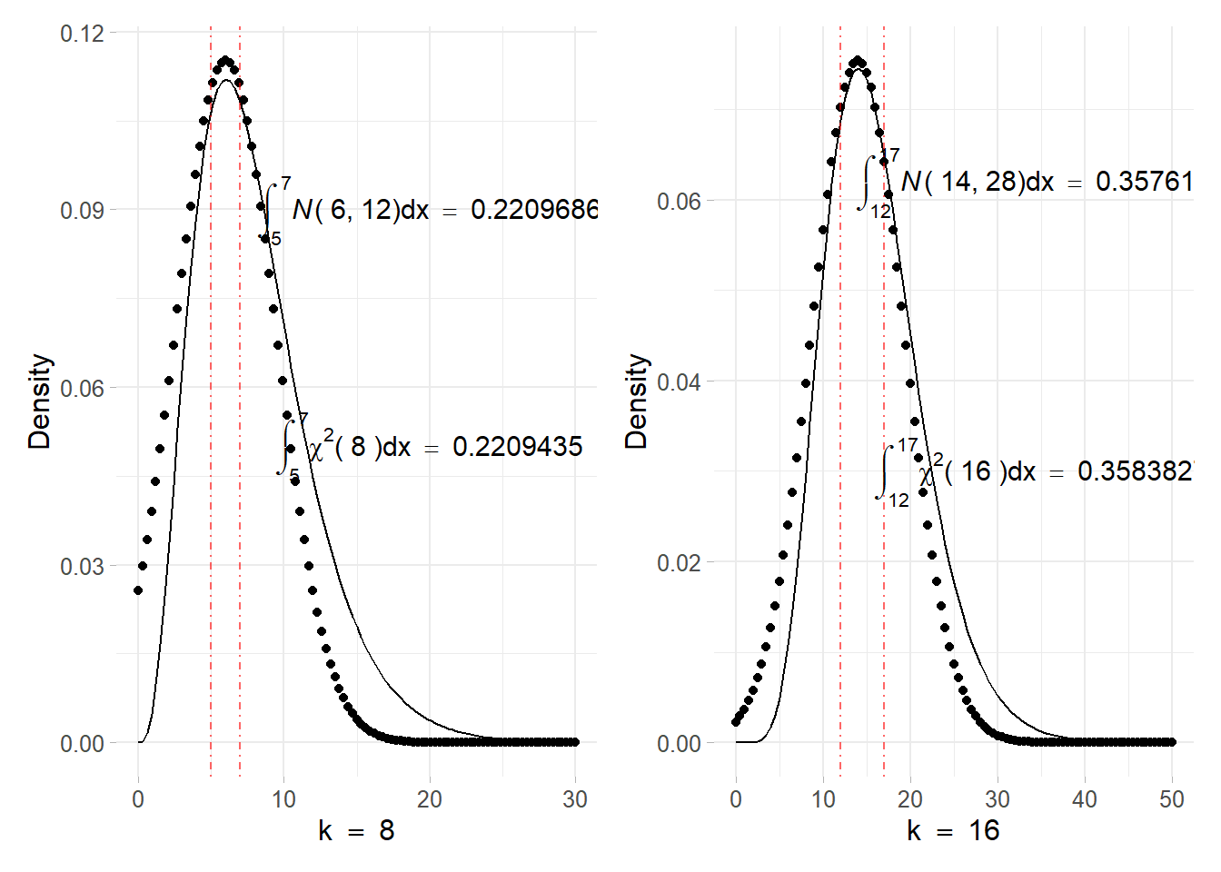
Figure 8.5: Chisquared density function with parameter \(k = 8\) (top) and \(k = 16\) (down) solid line. The point line refers to the corresponding Normal approximation obtained using the Laplace method
\[ \pi(\boldsymbol{\psi}) \quad \boldsymbol{\psi}= \boldsymbol{\psi_1}, \boldsymbol{\psi_2} \]