Chapter 6 Exploratory Analysis
To the analysis extent data should be constrained to the same geographic area and then saved otherwise the analysis would not be neither comparable nor reproducible since each time the API is called data gets updated. As a consequence the API is invoked with fixed request parameters by securing to the API the .thesis option, section 3.1.5. In other words the (mandatory) argument option guarantees to specify to the API an already pre-composed url to be passed to the scraping endpoint. The choice for this analysis is submitting the url corresponds to the properties restricted to a fixed set of micro-zones inside the circonvallazione i.e. beltway of Milan ( Municipality of Milan ). On the other side the resulting data is locally stored to be able to have consistent inference. (api parameters, number of covariates and number of observations)
Data emerging from the RESTful API response is not in its tidiest format. Yet data undergoes to a series of pre-processing steps during scraping, after which still requires to clear up unnecessary character and to separate columns containing more than one information. Therefore a summary table of the covariates, tab. 6.1, involved into the analysis is presented with the goal to familiarize with incoming API data. Data gathered from the second /completescrape endpoint contains geostatistical components and consequently a map representation of Real Estate rental maket at the gitbook building time i.e. 2021-06-14 is given. A further plot assess spatial dependence highlighting that coordinates are non-linearly related ?? to the y-response monthlyprice variable. Exploration starts with factor counts evidencing a “Bilocale” prevalence. This implies some critical Milan real estate market demand information and consequently reflections on the offer. Data displays bimodality in prices distribution for different n-roomed accommodations and the model should take account of the behavior. Then a piece-wise linear regression is fitted for each household type accommodation factor, whose single predictor is the square meter footage. The analysis emphasize some valuable economic consequences both for investors interested into property expansions and for tenants that are planning to partition single properties into rentable sub-units. The previous analysis brings along a major question which addresses the most valuable properties per single square meter surface and an answer based on data is given. Then a log-linear model is fitted on some presumably important covariates to evaluate each single house characteristic contribution to the price. A Tie Fighter plot displays for which coefficient, associated to each dummy predictor, are encountered surprisingly high monthly prices, compared to the effect of the square meter footage expansion. A partial conclusion is that disposing of 2 or 3+ bathrooms truly pays back an extra monthly return, also due to the number of tentants the accomodations could host. Text mining techniques are applied on real estate agency reviews and a network graph can help to distinguish topics. Then Missing assessement and imputation takes place. At first is made a brief a revision on randomness in missing by Little and Rubin (2014) which may help to figure out if data is missing due to API failures or for other reasons. Theory is applied by visualizing missingness in combination with heat-map and co-occurrence plot. Combined missing observation test is able to detect whether data is missing because of inner scraping faiilures or simple low prevalence in appereance. Then for each of the covariate that pass the exam, then imputation is made through INLA posterior expectation. This is the case of missing data in predictors, so the missing covariates ( condominium ) are brought into a model as response variable where this time predictors are the explanatory ones. Through a method specified within the INLA function the posterior statistics are computed and then finally imputed in the place of missing ones.
| name | descrition |
|---|---|
| id | ID of the apartements |
| lat | latitude coordinate |
| long | longitude coordinate |
| location | property address: street name and eventual number |
| condom | condominium monthly expenses |
| buildage | age in which the building was contructed |
| indivsapt | indipendent property type versus apartement type |
| locali | type and number of rooms |
| propcat | property category |
| status | maintenance status of the house, ristrutturato, nuovo, abitabile |
| heating | heating system |
| ac | air conditioning |
| catastinfo | land registry information |
| aptchar | apartement characteristics |
| photosnum | number of photos displayed in the advertisement |
| age | real estate agency name |
| enclass | energy class |
| contr | contract type proposed |
| disp | availability or already rented |
| totpiani | total number of building floors |
| postauto | number of parking box or garages |
| review | estate agency review (long chr string) |
| total_main_surface | total apartement surface area |
| total_commercial_surface | total commercial surface area |
| constitution | covered and uncovered surface areas type |
| floor | the property floor for each covered and uncovered area |
| surface | square meter footage for each covered and uncovered type |
| percentage | contribution percentage for each element to the total surface |
| surface_type | appliances or princpal category surface |
| commercial_surface | square meter footage for each commercial surface area |
| multi | it if has multimedia option, (3D house ristualization home experience and videos) |
| original_price | If the price is lowered it flags the starting price |
| current_price | If the price is lowered it flags the current price |
| passed_days | If the price is lowered marks the number of days passed by since the price change |
| date | the date of publication of the advertisement |
| nroom | number of rooms (int) |
| price | monthly price € (response) |
| sqfeet | total square meters footage surface area (int) |
| title | title of advertisement |
6.1 Preprocessing and Feature Engineering
Data needs to undergo to many previous cleaning preprocess steps, which mainly regard separating columns and extracting relevant covariates. This is a forced stage since for the way the API is designed it tries several searches (refer to fig. 2.7). Chances are that the search algorithm explores a hidden json object nested in the website source code, which actually needs to be properly wrangled. Steps followed are:
- locali needs to be separated, from which are drained out 5 categories : totlocali, camereletto, altro, bagno, cucina. nroom now is a duplicate for totlocali, so it is discarded.
- aptchar is a character string column that contains a non fixed number of features per house. The preprocess steps include cleaning the string from unnecessary characters, finding the set of unique elements across the character column (regex pattern), separating each feature in its proper column, in the end recoding newly created bivariate columns as “yes” or “no” according to a matching pattern.
- dropped unnecessary non UTF characters from continuous integer covariates i.e. price, condominium, sqfeet
- recoded factors for totlocali and floor
The previous steps lead to have a 250 data points per 64 covariates. Ultimately exploiting the spatial component, data can be represented through a map, as in fig. ??. Maps (not properly a “spatial” visualization) must determine the regularity of the arrangement of points and also if the maximum gap between points is much greater in some directions than others (symptomps of anisotropy, not detected).
6.2 Spatial Dependece Assessement
Spatial continuous data, as Waldo Tobler’s first law suggests, may be split split into a mean term and an error term (Banerjee, Carlin, and Gelfand 2014). The mean is the global (or first order) behaviour, while the error reports a contextual (or second-order) behavior through a covariance function. An effective set of EDA on spatial data should be able to separate and correctly detect these two quantities. As a matter of fact spatial data association for the spatial process \(Y(s)\) need not imitate its residuals \(\epsilon(s)\). A 3D scatterplot elevated for the price is plotted in 6.1, this is effective in displaying how the response is spatially dependent however it does not reveal the entire spatial surface. Moreover it can be tricky since it can display a spatial pattern that vanishes as soon as a model is fitted or vice versa. The analysis of spatial variations in the residual seems more organic (2014)
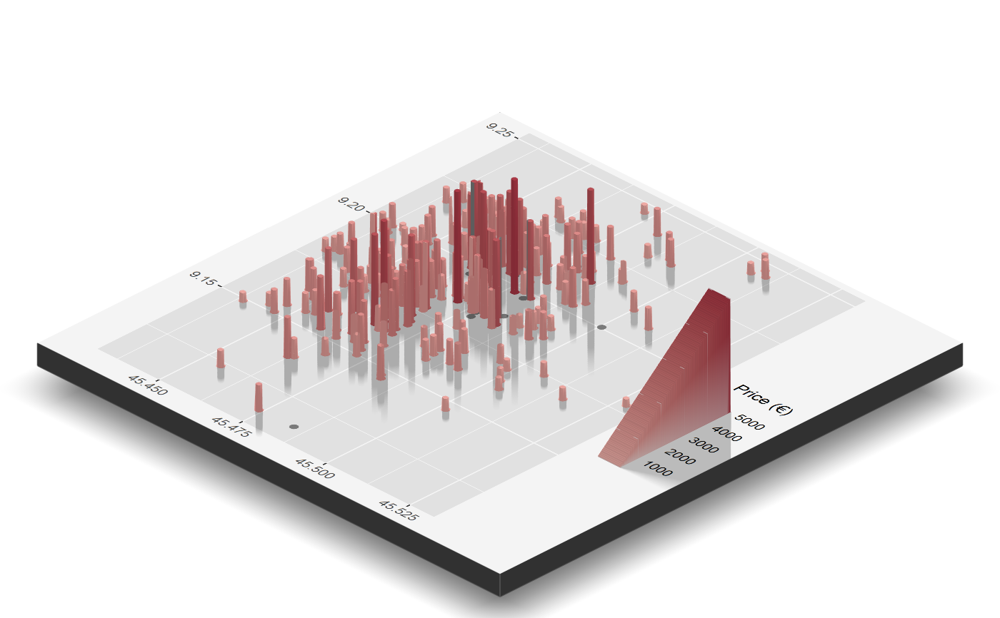
Figure 6.1: 3D Rayshader (rayshader?) Perspective scatterplot with Price elevation
By visual inspection, even though is assumed, the distribution of price seems to suffer for spatial dependence. In order to measure the range of spatial dependency and get an idea about the sill and nugget (seen in section 5.1 of previous chapter), further research is urged through a variogram analysis. The assessment continues by fitting an isotropical semivariogram with Matérn covariance 5.4 on residuals due to the assumption made before. Residuals are extracted from a regression model whose formula relates price with other presumably important covariates i.e. \(\text{price} \sim \text{totlocali} + \text{condominium}+ \text{sqmeter}\). The model is also computed through inla and by taking advantage of INLAtools and Pearson residuals (Cordeiro 2004) are extracted, i.e. \(\operatorname{Pearson}_{i}=\frac{y_{i}-\hat{y}_{i}}{\sqrt{M S E}}\). Moreover variogram from package gstat is versatile enough to allow to specify a regression model within the variogram function. The range parameter initial value is set equal to the maximum pair points distance registered.
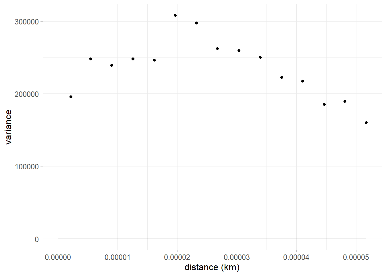
Figure 6.2: Semivariogram on a linear model Pearson residuals
6.3 Factor Counts
Arranged Counts for categorical columns can give a sense of the distribution of categories across the dataset suggesting also which predictors and which factor is relevant to the analysis. The left panel in figure 6.3 offers the rearranged factor count fot the covariate TOTLOCALI. “Bilocale” are the most common option for rent, then “Trilocale” follows. The intuition behind suggests that Milan rental market is oriented to “lighter” accommodations in terms of space and squarefootage. This comes natural since Milan is both a vivid study and working area, so temporary accommodations are warmly welcomed. Right in figure 6.3 it can be seen that building are generally old and mostly built either at the start of the 20th century or in the middle. Further investigation might assess how this fact can affect the overall city status.
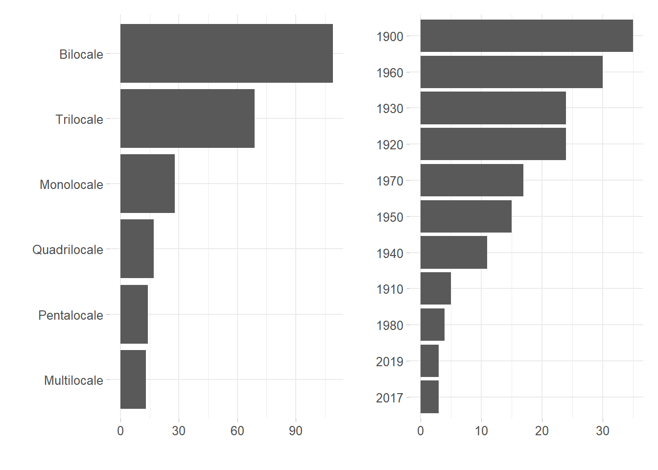
Figure 6.3: Left: Count plot for each housedolds category, Right: count plot for building age
Two of the most requested features for comfort and livability in rents are the heating/cooling systems. Moreover rental market demand, regardless of the rent duration, strives for a ready-to-accomodate offer to meet clients expectation. In this sense accommodation coming with the newest and the most technologically advanced systems are naturally preferred.
x-axis in figure 6.4 represents \(\log_{10}\) price for both of the upper and lower panel. Logarithmic scale is needed to smooth distributions and the resulting price interpretation have to considered into relative percent changes. Furthermore factors are reordered with respect to decreasing price.
y-axis are the different level for the categorical variables recoded from the original data due to simplify lables and to hold plot dimension. Moreover counts per level are expressed between brackets close to their respective factor.
The top plot displays the most prevalent heating systems categories, among which the most prevalent is “Cen_Rad_Met” by far. This fact is extremely important since methane is a green energy source and if the adoption is wide spread and pipelines are well organized than the city turns out to be sustainable. Indeed according to data there is still a 15% portion of houses powered by oil fired (old and polluting heating systems), which has been already presumed in the previous plot. This partially explains why Milan is one of the most polluted city in the world.
Then in bottom plot Jitters point out the number of outliers outside the IQR (Inter Quantile Range) .25 and their impact on the distribution. A first conclusion is that outliers are mainly located in autonomous systems, which leads of course to believe that the most expensive houses are heated by autonomoius heating systems. Indeed in any case this fact that does not affect monthly price. The overlapping IQR signifies that the covariates levels do not impact the response variable.
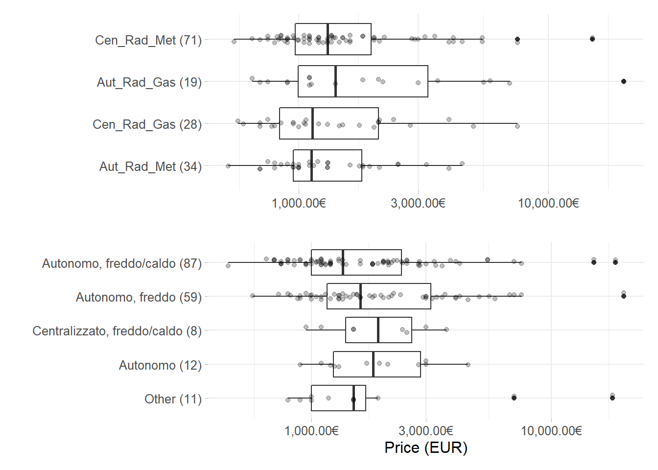
Figure 6.4: Log Monthly Prices box-plots for the most common factor levels in Heating systems and Air Conditionings
6.4 Assessing the most valuable properties
It might be relevant also to research how monthly prices change with respect to houses’ square footage for each house configuration, in other word how much adding a further square meter affects monthly price for each n-roomed flat. Answering to the previous question implies also knowing how properties should be developed in order to request a greater amount of money per month. This may be of interest, for instance, to those who have to lot their property into sub units and need to decide the most profitable choice in economic terms by setting ex ante the square footage extensions. A further example may regard the economic convenience for those who need to enlarge new properties (construction firms). Some of the potential enlargements are economically justified, some of the other are not. The plot 6.5 has two continuous variables for x (price) and y (sqfeet) axis, the former is once again \(log_{10}\) scaled. Coloration discretizes points for each of \(j_{th}\) totlocali. A sort of overlapping piece-wise linear regression (log-linear due to the transformation) is fitted on each totlocali group, whose response variable is price and whose only predictor is the square footage surface (i.e. \(\log_{10}(\text{price}_j) \sim +\beta_{0,j}+\beta_{1,j}\, \text{sqfeet}_j\)). Five different regression models are proposed in the top left. The interesting part regards the models slopes \(\hat\beta_{1,j}\). The highest corresponds to “Monolocale” for which the enlargement of a 10 square meters in surface enriches the apartment of a 0.1819524% monthly price addition. Almost the same is witnessed in “Bilocale” for which a 10 square meters extension gains a 0.1194379% value. One more major thing to notice is the “ensamble” regression line obtained as the interpolation of the 6 plotted ones. The line suggests a clear logarithmic pattern from Pentalocale and beyond whose assumption is strengthened by looking at the decreasing trend in the \(\hat\beta_1\) predictor slopes coefficients. Furthermore investing into an extension for “Quadrilocale” and “Trilocale” is coeteris paribus an interchangeable economic choice.
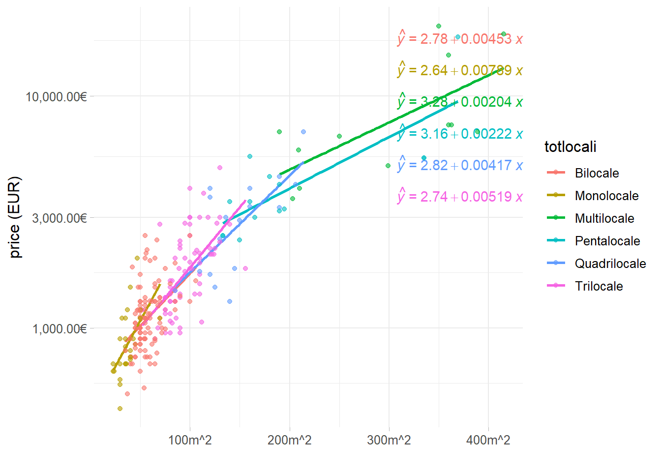
Figure 6.5: Monthly Prices change wrt square meters footage in different n-roomed apt
Furthermore in table 6.2 resides the answer to the question “which are the most profitable properties per square meter footage.” The covariate floor together with the address are not part of this simple regression model, indeed they can help explaining the behavior. First and third position are unsurprisingly “Bilocale.” The second stands out for its ridiculous price per month. The other are all located nearby the city center.
| location | totlocali | price | sqfeet | floor | totpiani | abs_price |
|---|---|---|---|---|---|---|
| via della spiga 23 | Bilocale | 2500 | 55 | 2 | 4 piani | 45.45€ |
| via dei giardini C.A. | Multilocale | 18500 | 415 | 2 | 6 piani | 44.58€ |
| piazza san babila C.A. | Bilocale | 1833 | 42 | 1 | 4 piani | 43.64€ |
| ottimo stato nono piano, C.A. | Monolocale | 2000 | 47 | 9 | 11 piani | 42.55€ |
| via tommaso salvini 1 | Multilocale | 15000 | 360 | 5 | 6 piani | 41.67€ |
| via cappuccini C.A. | Trilocale | 4000 | 100 | 3 | 5 piani | 40€ |
6.5 Assessing relevant predictors
Now it is fitted a log-linear model whose response is price and whose covariates are the newly created abs_price and some other presumably important ones e.g. floor, bagno, totpiani. The model formula is \(\log_{2}(price) \sim \log_{2}(abs\_price) + condominium + other_colors\). The plot in figure 6.6 has the purpose to demonstrate how monthly price is affected by covariates conditioned to their respective square meter footage. The interpretation of the plot starts by fixing a focus point on 0, which is the null effect highlighted by the red dashed line. Then the second focus is on house surface effect (i.e. House Surface (doubling) in the plot, the term \(\log_{2}(abs\_price)\) has been converted to more familiar House Surface (doubling)), which contributes to increase the price of an estimated coefficient of \(\approx .6\) for each doubling of the square meter footage. Then what it can be noticed with respect to the two focus points are the unusual effects provoked by the other predictors to the right of the doubling effect and to the far left below 0. “2 bagni,” 3 bagni" and 3+ bagni" are unusually expensive with respect to the square meter footage increment, on the other hand “al piano rialzato” and “al piano terra” are undervalued with respect to their surface. The fact that 2 and 3 bathrooms can guarantee a monthly extra check is probably caused to a minimum rent plateau requested for each occupant. the number of bathrooms are a proxy to both house extension since normally for each sleeping room there also exist at least 1 bathroom as well as prestigious houses dispose of more than 1 toilette services. So the more are the occupants regardless of the square meter footage dedicated to them, the more the house monthly returns.
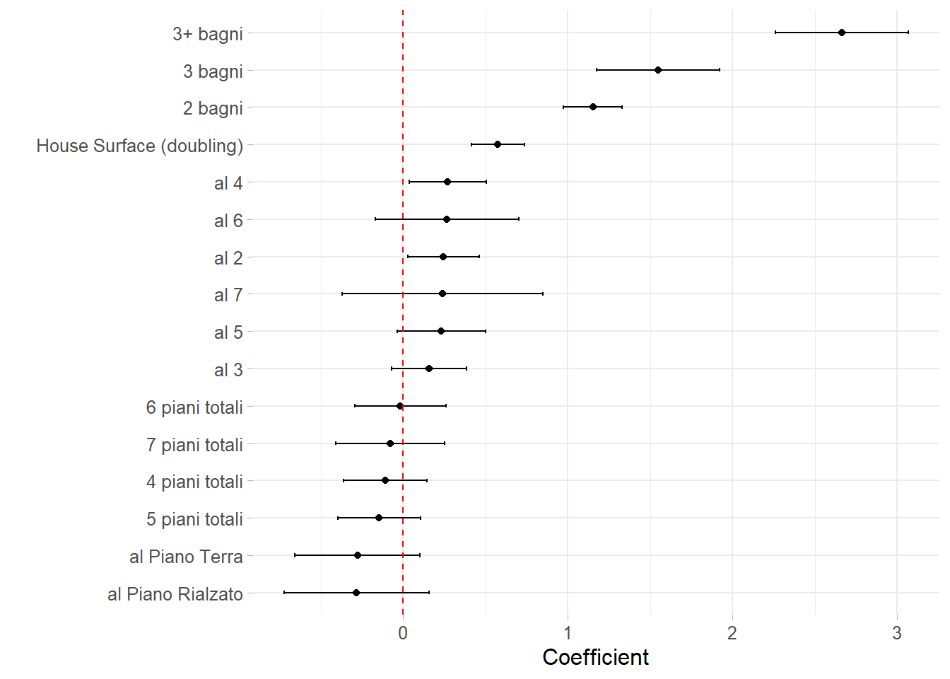
Figure 6.6: Tie fighter coefficient plot for the log-linear model
6.6 Missing Assessement and Imputation
Some data might be lost since immobiliare provides the information that in turn are pre filled by estate agencies or privates through standard document formats. Some of the missing can be traced back to scraping, some other are due to the context. The section tries to give substantial insights to discern what it can be recalled to the former issue or to the latter. The guidelines followed in this part is to prune redundant data and rare predictors trying to limit the dimensionality of the dataset as well as keeping covariates that are assumed to be relevant.
6.6.1 Missing Assessement
When data is presenting missing values, the analyst should typically investigate the etiology its lack (Kuhn and Johnson 2019). As already pointed out in the dedicated section 2.3 many of the presumably important covariates (i.e. price lat, long, title ,id …) undergo to a sequence of nested searches within the web page with the aim to avoid to be lost. This guarantees that when data is missing is actually due to an improper advertisement completion when posting the offer and by no means to a superficial scrape. Moreover empirical observation suggests that when relevant advertisement data is absent then it is more likely that the rest of the information are missing too. However in the API context the missing profile is crucial since it can also raise suspicion on scraping inability to catch data. By taking advantage of the patterns the maintainer can directly identify which data or combination of data are missing and immediately debug the error. In order to identify the nature of the missing patterns a revision of missing and randomness is introduced (Little and Rubin 2014). Categories are three:
- MCAR (Missing Completely At Random ), the likelihood of missing is equal for all the information, in other words missing data are one independent from the other.
- MAR (Missing At Random). the likelihood of missing is not equal.
- NMAR (Not Missing At Random), data that is missing due to a specific cause, scarping is an option.
This MNAR case is difficult to detect since the missing process and details are not available. An example of MNAR is the case of daily monitoring clinical studies (2019), when patient might drop out the experiment because of death, as a result all the subsequent data starting from the death time +1 are lost. Patterns are visible through a statistical tool whose typical application is found in detecting collinearity in predictors i.e. heat map. The plot in fig. 6.7 assign \(1\) when data is present and \(0\) otherwise. Gray background signifies data presence, black absence.
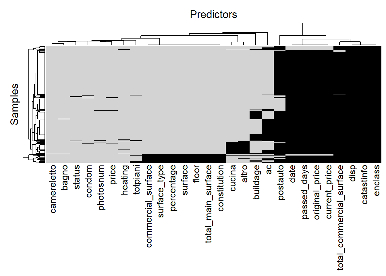
Figure 6.7: Heatmap of missing observations where gray implies data presence otherwise black, author’s source
Looking at the top of the heat map plot, the first tree split divides predictors into two sub-trees. The left branch considers from camereletto to ac and there are no evident patterns except for a small portion of the group from constitution to commercial surface. In the former group the missing pattern can be traced back to MAR and covariate imputation for condom, photosnum and price is scheduled (response and relevant continuous covariate). In the latter group a further inspection in the scraping code suggests that missing pattern are traced back to an improperly parsed json object in the source code, that is the case of NMAR and observations needs to be left out (covariate are not assumed to be important, therefore are not included in the model). From cucina to post_auto a relevant pattern is evident for cucina and altro, that is because they come from the same predictor from which have been feature engineered two separated and different covariates. As a result the observations that are missing for the one are also missing for the other. Nonetheless the entire group of covariates is dropped due to rarity (percentages of missing are found in tab. ??). In the far right side of figure 6.7 enclass, catastinfo and disp data are completely missing (NMAR), the pattern suggests some problem in gathering the respective values. A further assessement of the API totally absent covariates scraping is strongly advised. From total_commercial_surface to date, as in cooccurrence plot in figure 6.8, they are missing in combination for a total of 196 out of 250 cases, therefore are dropped, even though the pattern is NMAR, suggesting that are strongly tied in the scraping process.
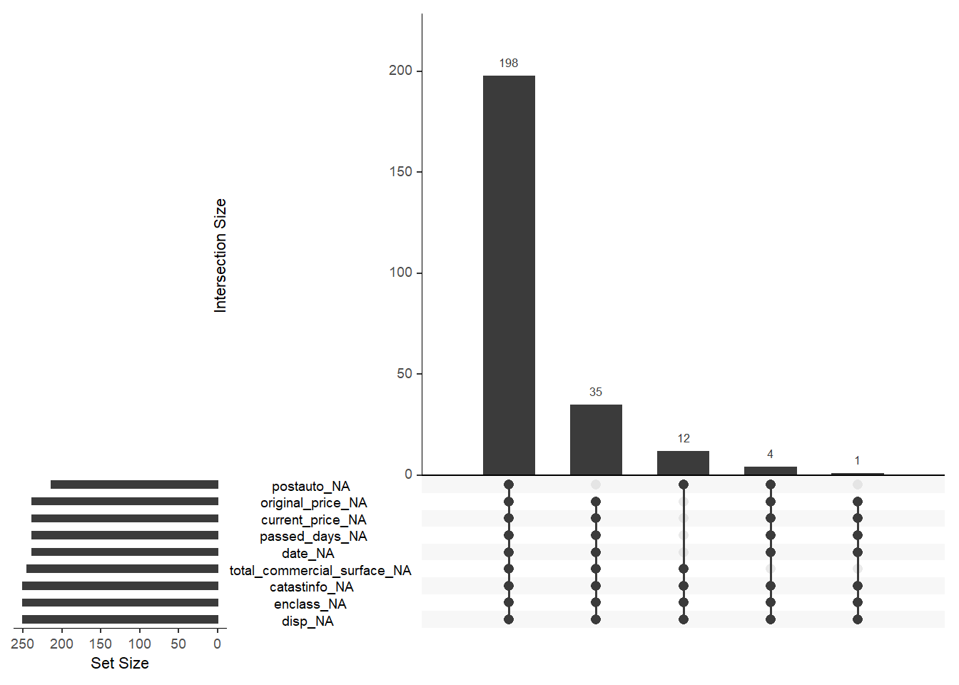
Figure 6.8: Missingness co-occurrence plot
6.6.2 Missing Imputation
A relatively simple approach to front MAR is to build a regression model to explain the covariates that contain missings and plug-back-in the respective posterior estimates (e.g. posterior means) from their predictive distributions Little and Rubin (2014). This approach is available in INLA and it is fast and easy to implement in most of the cases, indeed it ignores the uncertainty behind the imputed values (Gómez Rubio 2020). However it has the benefit to be a more than a reasonable choice with respect to the number of imputation needed. There are two approaches to follow, the former that considers the imputation of the response, the latter it has been designed for covariates. Since the response is not missing, indeed it does condominium, imputation is pursued for it. The output below reports the corresponding data indexes for missing observations in condominium.
#> [1] 83 109 132 167A model is fitted based on missing data for which the response variable is condominium and predictors are other important explanatory ones, i.e.\(condom ~ 1 + sqfeet + totlocali + floor + heating + ascensore\). In addition to the formula in the inla function a further specification has to be provided with the command compute = TRUE in the argument control.predictor. The command compute estimates the posterior means of the predictive distribution in the response variable for the missing points. The estimated posterior mean quantities are then imputed in place of the missing indexes. Results are in table @red(tab:condomimputation).
| mean | sd | |
|---|---|---|
| fitted.Predictor.083 | 129.8461 | 12.65487 |
| fitted.Predictor.109 | 233.6109 | 16.10042 |
| fitted.Predictor.132 | 312.9235 | 16.60390 |
| fitted.Predictor.167 | 106.9133 | 22.13250 |