Chapter 4 INLA

Bayesian estimation methods - by MCMC (Brooks et al. 2011) and MC simulation techniques - are usually much harder than Frequentist calculations (Wang, Yue, and Faraway 2018). This unfortunately is also more critical for spatial and spatio-temporal model settings (Cameletti et al. 2012) where matrices dimensions and densities (in the sense of prevalence of values throughout the matrix) start becoming unfeasible. The computational aspect refers in particular to the ineffectiveness of linear algebra operations with large dense covariance matrices that in aforementioned settings scale to the order $\mathcal{O}(n^3)$. INLA (Håvard Rue, Martino, and Chopin 2009; Håvard Rue et al. 2017) stands for Integrated Nested Laplace Approximation and constitutes a faster and accurate deterministic algorithm whose performance in time indeed scale to the order $\mathcal{O}(n)$. INLA is alternative and by no means substitute (Rencontres Mathématiques 2018) to traditional Bayesian Inference methods. INLA focuses on Latent Gaussian Models LGM (2018), which are a rich class including many regressions models, as well as support for spatial and spatio-temporal. INLA turns out to shorten model fitting time for essentially two reasons related to clever LGM model settings, such as: Gaussian Markov random field (GMRF) offering sparse matrices representation and Laplace approximation to approximate posterior marginals’ integrals with proper search strategies. In the end of the chapter it is presented the R-INLA project and the package focusing on the essential aspects. Further notes: the chronological steps followed in the methodology presentation retraces the canonical one by Håvard Rue, Martino, and Chopin (2009), which according to the author’s opinion is the most effective and the default one for all the related literature. The approach is more suitable and remains quite unchanged since it is top-down, which naturally fits the hierarchical framework imposed in INLA. The GMRF theory section heavily relies on Havard Rue and Held (2005).
Notation is imported from Michela Blangiardo Marta; Cameletti (2015) and integrated with Gómez Rubio (2020), whereas examples are drawn from Wang, Yue, and Faraway (2018). Vectors and matrices are typeset in bold i.e. $\boldsymbol{\beta}$, so each time they occur they have to be considered such as the ensamble of their values, whereas the notation $\beta_{-i}$ denotes all elements in $\boldsymbol{\beta}$ but $\beta_{-i}$. $\pi(\cdot)$ is a generic notation for the density of its arguments and $\tilde\pi(\cdot)$ has to be intended as its Laplace approximation. Furthermore Laplace Approximations mathematical details, e.g. optimal grid strategies and integration points, are overlooked instead a quick intuition on Laplace functioning is offered in the appendix 8.2.

4.1 The class of Latent Gaussian Models (LGM)

Bayesian theory is straightforward, but it is not always simple to measure posterior and other quantities of interest (Wang, Yue, and Faraway 2018). There are three ways to obtain a posterior estimate: by Exact estimation, i.e. operating on conjugate priors, but there are relatively few conjugate priors which are also employed in simple models. By Sampling through generating samples from the posterior distributions with MCMC methods (Metropolis et al. 1953; Hastings 1970) later applied in Bayesian statistics by Gelfand and Smith (1990). MCMCs have improved over time due to inner algorithm optimization as well as both hardware and software progresses, nevertheless for certain model combinations and data they either do not converge or take an unacceptable amount of time (2018). By Approximation through numerical integration and INLA can count on a strategy leveraging on three elements: LGMs, Gaussian Markov Random Fields (GMRF) and Laplace Approximations and this will articulates the steps according to which the arguments are treated. LGMs despite their anonymity are very flexible and they can host a wide range of models as regression, dynamic, spatial, spatio-temporal (Cameletti et al. 2012). LGMs necessitate further three interconnected elements: Likelihood, Latent field and Priors. To start it can be specified a generalization of a linear predictor $\eta_{i}$ which takes into account both linear and non-linear effects on covariates:

\[\begin{equation} \eta_{i}=\beta_{0}+\sum_{m=1}^{M} \beta_{m} x_{m i}+\sum_{l=1}^{L} f_{l}\left(z_{l i}\right) \tag{4.1} \end{equation}\]

where $\beta_{0}$ is the intercept, $\boldsymbol{\beta}=\left\{\beta_{1}, \ldots, \beta_{M}\right\}$ are the coefficients that quantifies the linear effects of covariates $\boldsymbol{x}=\left({x}_{1}, \ldots, {x}_{M}\right)$ and $f_{l}(\cdot), \forall l \in 1 \ldots L$ are a set of random effects defined in terms of a $\boldsymbol{z}$ set of covariates $\boldsymbol{z}=\left(z_{1}, \ldots, z_{L}\right)$ e.g. Random Walks (Havard Rue and Held 2005), Gaussian Processes (Besag and Kooperberg 1995), such models are termed as General Additive Models i.e. GAM or Generalized Linear Mixed Models GLMM (Wang, Yue, and Faraway 2018). For the response $\mathbf{y}=\left(y_{1}, \ldots, y_{n}\right)$ it is specified an exponential family distribution function whose mean $\mu_i$ (computed as its expectation $\left.E\left(\mathbf{y}\right)\right)$) is linked via a link function $\mathscr{g}(\cdot)$ to $\eta_{i}$ in eq. (4.1), i.e. $\mathscr{g}\left(\mu_i\right)=\eta_{i}$. At this point is possible to group all the latent (in the sense of unobserved) inference components into a variable, said latent field and denoted as $\boldsymbol{\theta}$ such that: $\boldsymbol{\theta}=\left\{\beta_{0}, \boldsymbol{\beta}, f\right\}$, where each single observation $i$ is connected to a $\theta_{i}$ combination of parameters in $\boldsymbol{\theta}$. The latent parameters $\boldsymbol{\theta}$ actually may depend on some hyper-parameters $\boldsymbol{\psi} = \left\{\psi_{1}, \ldots, \psi_{K}\right\}$. Then, given $\mathbf{y}$, the joint probability distribution function conditioned to both parameters and hyper-parameters, assuming conditional independence, is expressed by the likelihood:

\[\begin{equation} \pi(\boldsymbol{\mathbf{y}} \mid \boldsymbol{\theta}, \boldsymbol{\psi})=\prod_{i\ = 1}^{\mathbf{I}} \pi\left(y_{i} \mid \theta_{i}, \boldsymbol{\psi}\right) \tag{4.2} \end{equation}\]

The conditional independence assumption grants that for a general couple of conditionally independent $\theta_j$ and $\theta_i$, where $i \neq j$, the joint conditional distribution is factorized by $\pi\left(\theta_{i}, \theta_{j} \mid \theta_{-i, j}\right)=\pi\left(\theta_{i} \mid \theta_{-i, j}\right) \pi\left(\theta_{j} \mid \theta_{-i, j}\right)$ (Michela Blangiardo Marta; Cameletti 2015), i.e. the likelihood in eq:(4.2). The assumption constitutes a building block in INLA since as it will be shown later it will assure that there will be 0 patterns encoded inside matrices, implying computational benefits. Note also that the product index $i$ ranges from 1 to $\mathbf{I}$, i.e. $\mathbf{I} = \left\{1 \ldots n \right\}$. In the case when an observations are missing, i.e. $i \notin \mathbf{I}$, INLA automatically discards missing values from the model estimation (2020), this would be critical during missing values imputation sec. 6.6. At this point, as required by LGM, are needed to be imposed Gaussian priors on each linear effect and each model covariate that have either a univariate or multivaried normal density in order to make the additive $\eta_i$ Gaussian (2018). An example might clear up the setting requirement: let us assume to have a Normally distributed response and let us set the goal to specify a Bayesian Generalized Linear Model (GLM). Then the linear predictor can have this appearance $\eta_{i}=\beta_{0}+\beta_{1} x_{i 1}, \quad i=1, \ldots, n$, where $\beta_{0}$ is the intercept and $\beta_{1}$ is the slope for a general covariate $x_{i1}$. While applying LGM are needed to be specified Gaussian priors on $\beta_{0}$ and $\beta_{1}$, such that: $\beta_{0} \sim N\left(\mu_{0}, \sigma_{0}^{2}\right)$ and $\beta_{1} \sim N\left(\mu_{1}, \sigma_{1}^{2}\right)$, for which the latent linear predictor $\eta_i$ is $\eta_{i} \sim N\left(\mu_{0}+\mu_{1} x_{i 1}, \sigma_{0}^{2}+\sigma_{1}^{2} x_{i 1}^{2}\right)$. It can be illustrated by some linear algebra (2018) that $\boldsymbol{\eta}=\left(\eta_{1}, \ldots, \eta_{n}\right)^{\prime}$ is a Gaussian Process with mean structure $\mu$ and covariance matrix $\boldsymbol{Q^{-1}}$. The hyperparameters $\sigma_{0}^{2}$ and $\sigma_{1}^{2}$ are to be either fixed or estimated by taking hyperpriors on them. In this context $\boldsymbol{\theta}=\left\{\beta_{0}, \beta_{1}\right\}$ can group all the latent components and $\boldsymbol{\psi} = \left\{\sigma_{0}^{2},\sigma_{1}^{2}\right\}$ is the vector of Priors. For what it can be noticed there is a clear hierarchical relationship for which three different levels are seen: a higher level represented by the exponential family distribution function on $\mathbf{y}$, given the latent parameter and the hyper parameters. The medium by latent Gaussian random field with density function given some other hyper parameters. The lower by the joint distribution or a product of several distributions for which priors can be specified So letting be $\boldsymbol{\mathbf{y}}=\left(y_{1}, \ldots, y_{n}\right)^{\prime}$ at the higher level it is assumed an exponential family distribution function given a first set of hyper-parameters $\boldsymbol\psi_1$, usually referred to measurement error precision Michela Blangiardo Marta; Cameletti (2015)). Therefore as in (4.2),

\[\begin{equation} \pi(\boldsymbol{\mathbf{y}} \mid \boldsymbol{\theta}, \boldsymbol{\psi_1})=\prod_{i\ = 1}^{\mathbf{I}} \pi\left(y_{i} \mid \theta_{i}, \boldsymbol{\psi_1}\right) \tag{4.3} \end{equation}\]

At the medium level it is specified on the latent field $\boldsymbol\theta$ a latent Gaussian random field (LGRF), given $\boldsymbol\psi_2$ i.e. the rest of the hyper-parameters,

\[\begin{equation} \pi(\boldsymbol{\theta} \mid \boldsymbol{\psi_2})=(2 \pi)^{-n / 2}| \boldsymbol{Q(\psi_2)}|^{1 / 2} \exp \left(-\frac{1}{2} \boldsymbol{\theta}^{\prime} \boldsymbol{Q(\psi_2)} \boldsymbol{\theta}\right) \tag{4.4} \end{equation}\]

where $\boldsymbol{Q(\psi_2)}$ denotes positive definite matrix and $|\cdot|$ its determinant. $\prime$ is the transpose operator. The matrix $\boldsymbol{Q(\psi_2)}$ is called the precision matrix that outlines the underlying dependence structure of the data, and its inverse $\boldsymbol{Q(\cdot)}^{-1}$ is the covariance matrix (Wang, Yue, and Faraway 2018). In the spatial setting this would be critical since by a specifying a multivariate Normal distribution of eq. (4.4) it will become a GMRF. Due to conditional independence GMRF precision matrices are sparse and through linear algebra and numerical method for sparse matrices model fitting time is saved (Havard Rue and Held 2005). In the lower level priors are collected togheter $\boldsymbol\psi_ =\{ \boldsymbol\psi_1\ , \boldsymbol\psi_2\}$ for which are specified either a single prior distribution or a joint prior distribution as the product of its independent priors. Since the end goal is to find the joint posterior for $\boldsymbol\theta$ and $\boldsymbol\psi$, then given priors $\boldsymbol\psi$ it possible to combine expression (4.3) with (4.4) obtaining:

\[\begin{equation} \pi(\boldsymbol{\theta}, \boldsymbol{\psi} \mid \mathbf{y})\propto \underbrace{\pi(\boldsymbol{\psi})}_{\text {priors}} \times \underbrace{\pi(\boldsymbol\theta \mid \boldsymbol\psi)}_{\text {LGRM}} \times \underbrace{\prod_{i=1}^{\mathbf{I}} \pi\left(\mathbf{y} \mid \boldsymbol\theta, \boldsymbol{\psi}\right)}_{\text {likelihood }} \tag{4.5} \end{equation}\]

Which can be further solved following (Michela Blangiardo Marta; Cameletti 2015) as:

\[\begin{equation} \begin{aligned} \pi(\boldsymbol{\theta}, \boldsymbol{\psi} \mid y) & \propto \pi(\boldsymbol{\psi}) \times \pi(\boldsymbol{\theta} \mid \boldsymbol{\psi}) \times \pi(\mathbf{y} \mid \boldsymbol{\theta}, \boldsymbol{\psi}) \\ & \propto \pi(\boldsymbol{\psi}) \times \pi(\boldsymbol{\theta} \mid \boldsymbol{\psi}) \times \prod_{i=1}^{n} \pi\left(y_{i} \mid \theta_{i}, \boldsymbol{\psi}\right) \\ & \propto \pi(\boldsymbol{\psi}) \times|\boldsymbol{Q}(\boldsymbol{\psi})|^{1 / 2} \exp \left(-\frac{1}{2} \boldsymbol{\theta}^{\prime} \boldsymbol{Q}(\boldsymbol{\psi}) \boldsymbol{\theta}\right) \times \prod_{i}^{n} \exp \left(\log \left(\pi\left(y_{i} \mid \theta_{i}, \boldsymbol{\psi}\right)\right)\right) \end{aligned} \tag{4.6} \end{equation}\]

From which the two quantities of interest are the posterior marginal distribution for each element in the latent field and for each hyper parameter.

\[\begin{equation} \begin{aligned} \begin{array}{l} \pi\left(\theta_{i} \mid \boldsymbol{\mathbf{y}}\right)=\int \pi\left(\boldsymbol{\theta}_{i} \mid \boldsymbol{\psi}, \boldsymbol{\mathbf{y}}\right) \pi(\boldsymbol{\psi} \mid \boldsymbol{\mathbf{y}}) d \boldsymbol{\psi} \\ \pi\left(\boldsymbol{\psi}_{k} \mid \boldsymbol{\mathbf{y}}\right)=\int \pi(\boldsymbol{\psi} \mid \boldsymbol{\mathbf{y}}) d \boldsymbol{\psi}_{-k} \end{array} \end{aligned} \tag{4.7} \end{equation}\]

From final eq: (4.6) is derived Bayesian inference and INLA through Laplace can approximate posterior parameters distributions. Sadly, INLA cannot effectively suit all LGM’s. In general INLA depends upon the following supplementary assumptions (2018):

The hyper-parameter number $\boldsymbol\psi$ should be unpretentious, normally between 2 and 5, but not greater than 20.
When the number of observation is considerably high ($10^4$ to $10^5$), then the LGMR $\boldsymbol\theta$ must be a Gaussian Markov random field (GMRF).

4.2 Gaussian Markov Random Field (GMRF)

In the order to make INLA working efficiently the latent field $\boldsymbol\theta$ must not only be Gaussian but also Gaussian Markov Random Field (from now on GMRF). A GMRF is a genuinely simple structure: It is just random vector following a multivariate normal (or Gaussian) distribution (Havard Rue and Held 2005). However It is more interesting to research a restricted set of GMRF for which are satisfied the conditional independence assumptions (section 4.1), from here the term “Markov.” Expanding the concept of conditional independece let us assume to have a vector $\boldsymbol{\mathbf{x}}=\left(x_{1}, x_{2}, x_{3}\right)^{T}$ where $x_1$ and $x_2$ are conditionally independent given $x_3$, i.e. $x_{1} \perp x_{2} \mid x_3$. With that said if the objective is $x_3$, then uncovering $x_2$ gives no information on $x_1$. The joint density for $\boldsymbol{\mathbf{x}}$ is

\[\begin{equation} \pi(\boldsymbol{\mathbf{x}})=\pi\left(x_{1} \mid x_{3}\right) \pi\left(x_{2} \mid x_{3}\right) \pi\left(x_{3}\right) \tag{4.8} \end{equation}\]

Now let us assume a more general case of AR(1) exploiting the possibilities of defining $f_{1}(\cdot)$ function through the eq. (4.1). AR(1) is an autoregressive model of order 1 specified on the latent linear predictor $\boldsymbol\eta$ (notation slightly changes using $\eta$ instead of $\theta$ since latent components are few), with constant variance $\sigma_{\eta}^{2}$ and standard normal errors (2005; 2018). The model may have following expression:

\[ \eta_t=\phi \eta_{t-1}+\epsilon_{t}, \quad \epsilon_{t} \stackrel{\mathrm{iid}}{\sim} \mathcal{N}(0,1), \quad|\phi|<1 \] Where $t$ pedix is the time index and $\phi$ is the correlation in time. The conditional form of the previous equation can be rewritten when $t = 2 \ldots n$:

\[ \eta_{t} \mid \eta_{1}, \ldots, \eta_{t-1} \sim \mathcal{N}\left(\phi \eta_{t-1}, \sigma_{\eta}^{2}\right) \] Then let us also consider the marginal distribution for each $\eta_i$, it can be proven to be Gaussian with mean 0 and variance $\sigma_{\eta}^{2} /\left(1-\phi^{2}\right)$ (2018). Moreover the covariance between each general $\eta_{i}$ and $\eta_{j}$ is defined as $\sigma_{\eta}^{2} \rho^{|i-j|} /\left(1-\rho^{2}\right)$ which vanishes the more the distance $|i-j|$ increases. Therefore $\boldsymbol\eta$ is a Gaussian Process, whose proper definition is in ??, with mean structure of 0s and covariance matrix $\boldsymbol{Q}^{-1}$ i.e. $\boldsymbol{\eta} \sim N(\mathbf{0}, \boldsymbol{Q}^{-1})$. $\boldsymbol{Q}^{-1}$ is an $n \times n$ dense matrix that complicates computations. But by a simple trick it is possible to recognize that AR(1) is a special type of GP with sparce precision matrix which is evident by showing the joint distribution for $\boldsymbol\eta$

\[ \pi(\boldsymbol{\eta})=\pi\left(\eta_{1}\right) \pi\left(\eta_{2} \mid \eta_{1}\right) \pi\left(\eta_{3} \mid \eta_{1}, \eta_{2}\right) \cdots \pi\left(\eta_{n} \mid \eta_{n-1}, \ldots, \eta_{1}\right) \] whose precision matrix compared to its respective covariance matrix is:

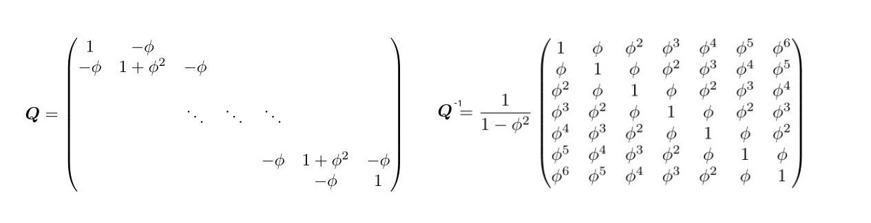
Figure 4.1: Precision Matrix in GMRF vs the Covariance matrix, source Havard Rue and Held (2005)

with zero entries outside the diagonal (right panel fig. 4.1) and first off-diagonals (2005). The conditional independence assumption makes the precision matrix tridiagonal since for generals $\eta_i$ and $\eta_j$ are conditionally independent for $|i − j| > 1$, given all the rest. In other words $\boldsymbol{Q}$ is sparse since given all the latent predictors in $\boldsymbol\eta$, then $\eta_t$ depends only on the preceding $\eta_{t-1}$. For example in (4.9), let assume to have $\eta_2$ and $\eta_4$, then:

\[\begin{equation} \begin{split} \pi\left(\eta_{2}, \eta_{4} \mid \eta_{1}, \eta_{3}\right) &=\pi\left(\eta_{2} \mid \eta_{1}\right) \pi\left(\eta_{4} \mid \eta_{1}, \eta_{2}, \eta_{3}\right) \\ & =\pi\left(\eta_{2} \mid \eta_{1}\right) \pi\left(\eta_{4} \mid \eta_{3}\right) \end{split} \tag{4.9} \end{equation}\]

For which the conditional density of $\eta_2$ does only depend on its preceding term i.e. $\eta_1$. The same inner reasoning can be done for $\eta_4$, which strictly depends on $\eta_3$ and vice versa. Therefore ultimately it is possible to produce a rather formal definition of a GMRF:

Definition 4.1 (GMRF) A latent gaussian random field (LGRM) e.g. $\boldsymbol\eta = \boldsymbol\theta$ (when $\mathscr{g}(\cdot)$ is identity) is said a GMRF if it has a multivariate Normal density with additional conditional independence (also called the “Markov property”) (Wang, Yue, and Faraway 2018).

\[ \pi(\boldsymbol{\theta} \mid \boldsymbol{\psi}_2) = \operatorname{MVN}(0, \boldsymbol{Q(\psi_2})) \]

4.3 INLA Laplace Approximations

The goals of the Bayesian inference are the marginal posterior distributions for each of the elements of the latent field. INLA is not going to try to approximate the whole joint posterior marginal distribution from expression (4.6) i.e. $\pi(\boldsymbol{\theta} \mid \boldsymbol{\psi}, \boldsymbol{\mathbf{y}})$, in fact if it would (two-dimensional approx) it will cause a high biased approximations since it fail to capture both location and skewness in the marginals. Instead INLA algorithm will try to estimate the posterior marginal distribution for each $\theta_{i}$ in the latent parameter $\boldsymbol{\theta}$, for each hyper-parameter prior $\psi_{k} \in \boldsymbol\psi$ (back to the $\boldsymbol\theta$ latent field notation).

The mathematical intuition behind Laplace Approximation along with some real life cases are contained in the appendix in sec. 8.2.

Therefore the key focus of INLA is to approximate with Laplace only densities that are near-Gaussian (2018) or replacing very nested dependencies with their more comfortable conditional distribution which ultimately are “more Gaussian” than the their joint distribution. Into the LGM framework let us assume to observe $n$ counts, i.e. $\mathbf{y} = y_i = 1,2, \ldots, n$ drawn from Poisson distribution whose mean is $\lambda_i, \forall i \in \mathbf{I}$. Then a the link function $\mathscr{g}(\cdot)$ is the $\log()$ and relates $\lambda_i$ with the linear predictor and so the latent filed $\theta$, i.e. $\log(\lambda_i)=\theta_{i}$. The hyper-parameters are $\boldsymbol\psi = (\tau, \rho)$ with their covariance matrix structure. \[ Q_{\psi}=\boldsymbol\tau\begin{bmatrix} 1 & - \rho & - \rho^{2} & - \rho^{3} & \ldots & - \rho^{n} & \\ - \rho & 1 & - \rho & - \rho^{2} & - \rho^{3} & - \rho^{n-1} & \\ - \rho^{2} & - \rho & 1 & - \rho & - \rho^{2} & - \rho^{n-2} & \\ - \rho^{3} & - \rho^{2} & - \rho & 1 & - \rho & - \rho^{n-3} & \\ - \ldots & - \rho^{3} & - \rho^{2} & - \rho & 1 & - \rho & \\ - \rho^{n} & - \rho^{n-1} & - \rho^{n-2} & - \rho^{n-3} & - \rho & 1 \\ \end{bmatrix} \]

Let us also to assume once again to model $\boldsymbol\theta$ with an AR(1). Then fitting the model into the LGM, at first requires to specify an exponential family distribution function, i.e. Poisson on the response $\mathbf{y}$. then the higher level (recall last part sec. 4.1) results in:

\[ \pi(\boldsymbol{\mathbf{y}} \mid \boldsymbol{\theta} , \boldsymbol{\psi}) \propto\prod_{i=1}^{\mathbf{I}} \frac{ \exp \left(\theta_{i} y_{i}-e^{\theta_{i}}\right) }{y_{i} !} \]

Then the medium level is for the latent Gaussian Random Field a multivariate gaussian distribution $\boldsymbol{\psi}_{i} \sim \operatorname{MVN}_{2}(\mathbf{0}, \boldsymbol{Q}_{\boldsymbol{\psi}})$:

\[ \pi(\boldsymbol{\theta} \mid \boldsymbol{\psi}) \propto\left|\boldsymbol{Q}_{\boldsymbol{\psi}}\right|^{1 / 2} \exp \left(-\frac{1}{2} \boldsymbol{\theta}^{\prime} \boldsymbol{Q}_{\boldsymbol{\psi}} \boldsymbol{\theta}\right) \] and the lower, where it is specified a joint prior distribution for $\boldsymbol\psi = (\tau, \rho)$, which is $\pi(\boldsymbol\psi)$. Following eq.(4.5) then:

\[\begin{equation} \pi(\boldsymbol{\theta}, \boldsymbol{\psi} \mid \mathbf{y})\propto \underbrace{\pi(\boldsymbol{\psi})}_{\text {priors}} \times \underbrace{\pi(\boldsymbol\theta \mid \boldsymbol\rho)}_{\text {GMRF}} \times \underbrace{\prod_{i=1}^{\mathbf{I}} \pi\left(\mathbf{y} \mid \boldsymbol\theta, \boldsymbol{\tau}\right)}_{\text {likelihood }} \tag{4.10} \end{equation}\]

Then recalling the goal for Bayesian Inference, i.e.approximate posterior marginals for $\pi\left(\theta_{i} \mid \mathbf{y}\right)$ and $\pi\left(\tau \mid \boldsymbol{\mathbf{y}}\right)$ and $\pi\left(\rho \mid \boldsymbol{\mathbf{y}}\right)$. First difficulties regard the fact that Laplace approximations on this model implies the product of a Gaussian distribution and a non-gaussian one. As the INLA key point suggest, the algorithm starts by rearranging the problem so that the “most Gaussian” are computed at first. Ideally the method can be generally subdivided into three tasks. At first INLA attempts to approximate $\tilde{\pi}(\boldsymbol{\psi} \mid \boldsymbol{\mathbf{y}})$ as the joint posterior of ${\pi}(\boldsymbol{\psi} \mid \boldsymbol{\mathbf{y}})$. Then subsequently will try to approximate $\tilde{\pi}\left(\theta_{i} \mid \boldsymbol\psi, \mathbf{y}\right)$ to their conditional marginal distribution fro $\theta_i$. In the end explores $\tilde{\pi}(\boldsymbol{\psi} \mid \boldsymbol{\mathbf{y}})$ with numerical methods for integration. The corresponding integrals to be approximated are:

for task 1: $\pi\left(\psi_{k} \mid \boldsymbol{\mathbf{y}}\right)=\int \pi(\boldsymbol{\psi} \mid \boldsymbol{\mathbf{y}}) \mathrm{d} \boldsymbol{\psi}_{-k}$
for task 2: $\pi\left(\theta_{i} \mid \boldsymbol{\mathbf{y}}\right)=\int \pi\left(\theta_{i}, \boldsymbol{\psi} \mid \boldsymbol{\mathbf{y}}\right) \mathrm{d} \boldsymbol{\psi}=\int \pi\left(\theta_{i} \mid \boldsymbol{\psi}, \boldsymbol{\mathbf{y}}\right) \pi(\boldsymbol{\psi} \mid \boldsymbol{\mathbf{y}}) \mathrm{d} \boldsymbol{\psi}$

As a result the approximations for the marginal posteriors are at first:

\[\begin{equation} \tilde{\pi}\left(\theta_{j} \mid \boldsymbol{\mathbf{y}}\right)=\int \tilde{\pi}(\boldsymbol{\theta} \mid \boldsymbol{\mathbf{y}}) d \boldsymbol{\theta}_{-j} \tag{4.11} \end{equation}\]

and then,

\[\begin{equation} \tilde{\pi}\left(\theta_{i} \mid \boldsymbol{\mathbf{y}}\right) \approx \sum_{j} \tilde{\pi}\left(\theta_{i} \mid \boldsymbol{\psi}^{(j)}, \boldsymbol{\mathbf{y}}\right) \tilde{\pi}\left(\boldsymbol{\psi}^{(j)} \mid \boldsymbol{\mathbf{y}}\right) \Delta_{j} \tag{4.12} \end{equation}\]

Where in the integral in (4.12) $\{\boldsymbol{\psi}^{(j)}\}$ are some relevant integration points and $\{\Delta_j\}$ are weights associated to the set of hyper-parameters ina grid. (Michela Blangiardo Marta; Cameletti 2015). In other words the bigger the $\Delta_{j}$ weight the more relevant are the integration points. Details on how INLA finds those points is beyond the scope, an indeep resource if offered by Wang, Yue, and Faraway (2018) in sec. 2.3.

4.4 R-INLA package

INLA library and algorithm is developed by the R-INLA project whose package is available on their website at their source repository. Users can also enjoy on INLA website (recently restyled) a dedicated forum where discussion groups are opened and an active community is keen to answer. Moreover It also contains a number of reference books, among which some of them are fully open sourced. INLA is available for any operating system and it is built on top of other libraries still not on CRAN. The core function of the package is inla()and it works as many other regression functions like glm(), lm() or gam(). Inla function takes as argument the model formula i.e. the linear predictor for which it can be specified a number of linear and non-linear effects on covariates as seen in eq. (4.1), the whole set of available effects are obtained with the command names(inla.models()$latent). Furthermore it requires to specify the dataset and its respective likelihood family, equivalently names(inla.models()$likelihood). Many other methods in the function can be added through lists, such as control.family and control.fixed which let the analyst specifying parameter and hyper-paramenters priors family distributions and control hyper parameters. They come in the of nested lists when parameters and hyper paramenters are more than 2, when nothing is specified the default option is non-informativeness. Inla output objects are inla.dataframe summary-lists-type containing the results from model fitting for which a table is given in figure 4.3.

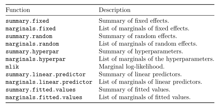
Figure 4.3: outputs for a inla() call, source: E. T. Krainski (2019)

SPDEtoy dataset $\mathbf{y}$ are two random variables that simulates points location in two coordinates $s_1$ and $s_2$.

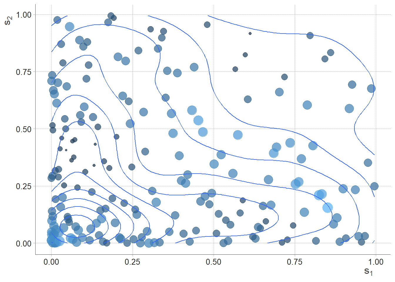
Figure 4.4: SPDEtoy bubble plot, author’s source

Imposing an LGM model requires at first to select as a higher hierarchy level a likelihood model for $\mathbf{y}$ i.e. Gaussian (by default), and a model formula (eq. (4.1)), i.e. $\eta_{i}=\beta_{0}+\beta_{1} s_{1 i}+\beta_{2} s_{2 i}$, which link function $\mathbf{g}$ is identity. There are not Non-linear effects effect on covariates in $$ nevertheless they can be easily added with f() function. Note that this will allow to integrate random effects i.e. spatial effects inside the model. Secondly in the medium step a LGRF on the latent parameters $\boldsymbol\theta$. In the lower end some priors distributions $\boldsymbol\psi$ which are Uniform for the intercept indeed Gaussian vagues (default) priors i.e. centered in 0 with very low standard deviation. Furthermore the precision hyper parameter $\tau$ which accounts for the variance of the latent GRF, is set as Gamma distributed with parameters $\alpha = 1$ and $\beta = 0.00005$ (default). Note that models are sensitive to prior choices (sec. 5.5), as a consequence if necessary later are revised. A summary of the model specifications are set below:

\[\begin{equation} \begin{split} y_{i} & \sim N\left(\mu_{i}, \tau^{-1}\right), i=1, \ldots, 200 \\ \mu_{i} &=\beta_{0}+\beta_{1} s_{1 i}+\beta_{2} s_{2 i} \\ \beta_{0} & \sim \text { Uniform } \\ \beta_{j} & \sim N\left(0,0.001^{-1}\right), j=1,2 \\ \tau & \sim G a(1,0.00005) \end{split} \end{equation}\]

Then the model is fitted within inla() call, specifying the formula, data and the exponential family distribution.

formula <- y ~ s1 + s2
m0 <- inla(formula, data = SPDEtoy, family = "gaussian")

Table 4.1 offers summary of the posterior marginal values for intercept and covariates’ coefficients, as well as precision. Marginals distributions both for parameters and hyper-parameters can be conveniently plotted as in figure 4.6. From the table it can also be seen that the mean for $s_2$ is negative, so the Norther the y-coordinate, the less is response. That is factual looking at the SPDEtoy contour plot in figure 4.4 where bigger bubbles are concentrated around the origin.

Table 4.1: Summary Posterior quantiles for coefficients
coefficients	mean	sd
(Intercept)	10.1321487	0.2422118
s1	0.7624296	0.4293757
s2	-1.5836768	0.4293757

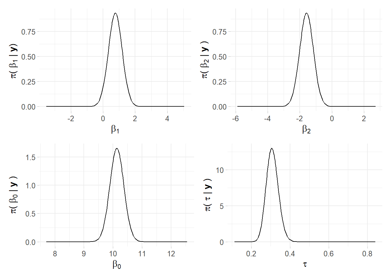
Figure 4.6: Linear predictor marginals, plot recoded in ggplot2, author’s source

In the end R-INLA enables also r-base fashion function to compute statistics on marginal posterior distributions for the density, distribution as well as the quantile function respectively with inla.dmarginal, inla.pmarginal and inla.qmarginal. One option which allows to compute the higher posterior density credibility interval inla.hpdmarginal for a given covariate’s coefficient i.e, $\beta_2$, such that $\int_{q_{1}}^{q_{2}} \tilde{\pi}\left(\beta_{2} \mid \boldsymbol{y}\right) \mathrm{d} \beta_{2}=0.90$ (90% credibility), whose result is in table below.

Table 4.2: Higer Posterior Density Interval for s2 coefficient
	low	high
level:0.9	-2.291268	-0.879445

Note that the interpretation is more convoluted (2018) than the traditional frequentist approach: in Bayesian statistics $\beta_{j}$ comes from probability distribution, while frequenstists considers $\beta_{j}$ as fixed unknown quantity whose estimator (random variable conditioned to data) is used to infer the value (2015).