Chapter 7 Model Selection & Fitting
In this chapter it is applied all the theory seen so far through the lenses of R-INLA package on the scraped data. The hierarchical Latent Gaussian model to-be-fitted sets against the response monthly price with the other predictors scraped. As a consequence on top of the hierarchy i.e. the higher level the model places the likelihood of data for which a Normal distribution is specified. At the medium level the GMRF containing the latent components and distributed as a Multivariate Normal (centered in zero and with “markov” properties encoded in the precision matrix). In the end priors are specified both for measurement error precision and for the latent field (penalized in complexity) i.e. the variance of the spatial process and the Matérn hyper parameters. The SPDE approach trinagularize the spatial domain and makes possible to pass from a discrete surface to a continuous representation of the own process. This requires a series of steps ranging from mesh building, passing the mesh inside the Matérn obtaining the spde object and then reprojecting through the stack function. In the end the model is fitted integrating the spatial random field. Posterior distributions for parameters and hyper parameters are then evaluated and summarized.
In order to make the distribution of the response i.e. price (per month in €) approximately Normal it is applied a \(log_{10}\) transformation (further transformation would have better Normalized data i.e. Box-Cox (Box and Cox 1964) and Yeo-Johnson (Yeo and Johnson 2000) however they over complicate interpretability). Moreover all of the numerical covariates e.g. condominium, sqmeter and photosnum have already been prepared in 6.1 and are further standardized and scaled. The Locations are represented in map plot 7.1 within the borders of the Municipality of Milan. At first the borders shapefile is imported from GeoPortale Milano. The corresponding CRS is in UTM (i.e. Eastings and Northings) which differs from the spatial covariates extracted (lat and long). Therefore the spatial entity needs to be rescaled and reprojected to the new CRS. In the end the latitude and the longitude points are overlayed to the borders as in figure 7.1.
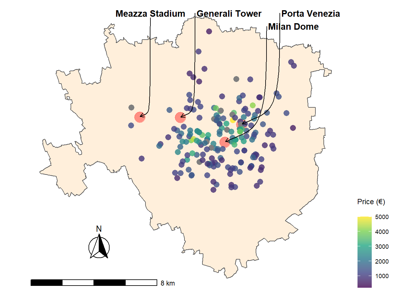
Figure 7.1: Milan Real Estate data within the Municpality borders, 4 points of interest
7.1 Model Specification & Mesh Assessement
WIth the aim to harness INLA power a hierarchical LGM need to be imposed. Its definition starts from fitting an exponential family distribution on Milan Real Estate Rental data \(\mathbf{y}\) i.e. normal distribution:
\[ \mathbf{y}\sim \operatorname{Normal}\left(\boldsymbol\mu, \sigma_{e}^{2}\right) \]
Then the linear predictor i.e. the mean, since the function \(\mathrm{g}\left(\boldsymbol\mu\right)\) is identity, is:
\[ \boldsymbol\eta=b_{0}+\boldsymbol x \boldsymbol\beta+\boldsymbol\xi \] where, following the notation in expression (4.1), \(\boldsymbol\xi\) is the spatial random effect assigned to the function \(f_1()\), for the set of coviarates \(\boldsymbol{z}=\left(x_{1} = lat,\, x_{2} = long\right)\). \(\boldsymbol\xi\) is also the GMRF defined in4.1, as a result it is distributed as a multivariate Normal centered in 0 and whose covariance function is Matérn (fig. 5.4) i.e. \(\xi_{i} \sim N\left(\mathbf{0}, \mathbf{Q}_{\mathscr{C}}^{-1}\right)\). The precision matrix \(\mathbf{Q}_{\mathscr{C}}^{-1}\) (see left panel in figure 4.1) is the one that requires to be treated with SPDE and its dimensions are \(n \times n\), in this case when NAs are omitted and after imputation it results in \(192 \times 192\). \(\boldsymbol\beta\) are the model scraped covariates coefficients. Then the latent field is composed by \(\boldsymbol{\theta}=\{\boldsymbol{\xi}, \boldsymbol{\beta}\}\). In the end following the traits of the final expression in 5.1 the LGM can be reformatted as follows,
\[ \boldsymbol{\mathbf{y}}=\boldsymbol{z} \boldsymbol{\beta}+\boldsymbol{\xi}+\boldsymbol{\varepsilon}, \quad \boldsymbol{\varepsilon} \sim N\left(\mathbf{0}, \sigma^2_{\varepsilon} I_{d}\right) \] Priors are assigned as Gaussian vagues ones for the \(\boldsymbol\beta\) coefficients with fixed precision, indeed for the GMRF priors are assigned to the matérn process \(\tilde{\boldsymbol\xi}\) as Penalized in Complexity. Thus following the steps and notation marked in sec. 4.1. the higher level eq. (4.3) is constituted by the likelihood, depending on hyper parameters \(\boldsymbol\psi_1 = \{\sigma_{\varepsilon}^2\}\):
\[\pi(\boldsymbol{\mathbf{y}} \mid \boldsymbol{\theta}, \boldsymbol{\psi_1})=\prod_{i\ = 1}^{\mathbf{192}} \pi\left(y_{i} \mid \theta_{i}, \boldsymbol{\psi_1}\right)\]
At the medium level eq. (4.4) there exists the latent field \(\pi(\boldsymbol{\theta} \mid \boldsymbol\psi_2)\), conditioned to the hyper parameter , whose only component is the measurement error precision, \(\boldsymbol\psi_2 = \left(\sigma_{\mathscr{\xi}}^{2}, \phi, \nu\right)\):
\[ \pi(\boldsymbol{\theta} \mid \boldsymbol{\psi_2})=(2 \pi)^{-n / 2}| \boldsymbol{Q_{\mathscr{C}}(\psi_2)}|^{1 / 2} \exp \left(-\frac{1}{2} \boldsymbol{\theta}^{\prime} \boldsymbol{Q_{\mathscr{C}}(\psi_2)} \boldsymbol{\theta}\right)\]
In the lower level priors are considered as their joint distribution i.e. \(\boldsymbol\psi_ =\{ \boldsymbol\psi_1\, \boldsymbol\psi_2\}\). It follows the expression of the joint posterior distribution:
\[ \pi(\boldsymbol{\theta}, \boldsymbol{\psi} \mid \mathbf{y})\propto \underbrace{\pi(\boldsymbol{\psi})}_{\text {priors}} \times \underbrace{\pi(\boldsymbol\theta \mid \boldsymbol\psi)}_{\text {GMRF}} \times \underbrace{\prod_{i=1}^{\mathbf{192}} \pi\left(\mathbf{y} \mid \boldsymbol\theta, \boldsymbol{\psi}\right)}_{\text {likelihood }} \] Then once again the objectives of bayesian inference are the posterior marginal distributions for the latent field and the hyperparameters, which are contained in equation (4.7), for which Laplace approximations in 4.3 are employed.
7.2 Building the SPDE object
SPDE requires to triangulate the domain space \(\mathscr{D}\) as intuited in 5.2. The function inla.mesh.2d together with the inla.nonconvex.hull are able to define a good triangulation since no proper boundaries are provided. Four meshes are produced, whose figures are in 7.2. Triangles appears to be thoroughly smooth and equilateral. The extra offset prevents the model to be affected by boundary effects. However the maximum accessible number of vertices is in \(\operatorname{mesh}_3\) , it seems to have the most potential for this dataset. Critical parameters for meshes are max.edge=c(0.01, 0.02) and offset=c(0.0475, 0.0625)) which in fact mold their sophistication. Further trials have shown that below the lower bound of max.edge of \(0.01\) the function is not able to produce the triangulation.
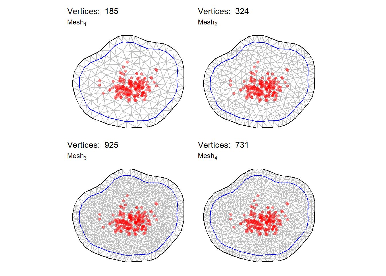
Figure 7.2: Left: mesh traingulation for 156 vertices, Right: mesh traingulation for 324 vertices
The SPDE model object is built with the function inla.spde2.pcmatern() which needs as arguments the mesh triangulation, i.e. \(\operatorname{mesh}_3\) and the PC priors 5.5, satisfying the following probability statements: \(\operatorname{Prob}(\sigma_{\varepsilon}^2<3060)< 0.01\) where \(\sigma_{\varepsilon}^2\) is the spatial range desumed in 6.2. And \(\operatorname{Prob}(\tau> 0.9)< 0.05\) where \(\tau\) is the marginal standard deviation (on the log scale) of the field 6.2.
As model complexity increases, for instance, a lot of random effects may be discovered in the linear predictor and chances are that SPDE object may get into trouble. As a result the inla.stack function recreates the linear predictor as a combination of the elements of the old linear predictor and the matrix of observations. Further mathematical details about the stack are in Michela Blangiardo Marta; Cameletti (2015), but are beyond the scope of the analysis.
7.3 Model Selection
Since covariates are many they arouse also many possible combinations of predictors that may better shape complex dynamics. However, there is the possibility to take advantage of several natively implemented ways to use built-in INLA features. As a matter of fact in section 5.4.2 are presented a set of tools to compare models based on deviance criteria. One of them is DIC which actually balances the number of features applying a penalty when the number of features introduced increases eq. (5.1). Consequently a Forward Stepwise Selection (Guyon and Elisseeff 2003) algorithm is designed within the inla function call. One at a time predictors are introduced into the model then results are stored into a dataframe. In the end the most satisfying combination based on DIC is sorted out.
#> [1] "condom + totlocali + bagno + cucina + heating + photosnum + floor + sqfeet + fibra_ottica + videocitofono + impianto_di_allarme + reception + porta_blindata WAIC = -7.532 DIC =-9.001"7.4 Parameter Estimation and Results
Now the candidate statistical model is fitted rebuilding the stack and calling inla on the final formula i.e. number of predictors. When the model has run, the conclusions for the random and fixed effects are now discussed.
| coefficients | mean | sd | 0.025quant | 0.5quant | 0.975quant |
|---|---|---|---|---|---|
| Intercept | 5.46 | 12.91 | -19.89 | 5.46 | 30.79 |
| totlocaliTrilocale | 1.19 | 12.91 | -24.15 | 1.19 | 26.52 |
| totlocali5+ | 1.18 | 12.91 | -24.17 | 1.18 | 26.50 |
| totlocaliBilocale | 1.09 | 12.91 | -24.25 | 1.09 | 26.42 |
| totlocaliQuadrilocale | 1.03 | 12.91 | -24.32 | 1.03 | 26.36 |
| totlocaliPentalocale | 0.97 | 12.91 | -24.38 | 0.97 | 26.29 |
| heatingAutonomo, a pavimento, alimentato a pompa di calore | 0.67 | 0.21 | 0.26 | 0.66 | 1.08 |
| receptionyes | 0.46 | 0.16 | 0.14 | 0.46 | 0.78 |
| heatingCentralizzato, ad aria | 0.33 | 0.17 | 0.00 | 0.33 | 0.66 |
| heatingCentralizzato, a pavimento, alimentato a pompa di calore | 0.31 | 0.15 | 0.01 | 0.31 | 0.60 |
Since the models coefficients are many i.e.66 the analysis will concentrate on the most interesting ones. Looking at table 7.1 where coefficients are arranged by descending mean, the posterior mean for the intercept, rescaled back from log, is truly quite lofty, affirming that the average house price is 235.1 €. Moreover being a “Trilocale” or “Bilocale,” as pointed out in 6.4, brings a monthly extra profit respectively of 3.29 € and 2.97 €. However standard deviations are quite high. Unsurprisingly the covariate condominium is positively correlated with the response price but its effect is not very tangible. This might imply that pricier apartments expect in mean the same condominium cost as the cheaper ones. Moreover one feature strongly requested and paid is having a floor heating system, regardless of it is autonomous or centralized. INLA is able to output the mean and the standard deviation of measurement precision error in \(\psi_2\) i.e. \(1 / \sigma_{\varepsilon}^{2}\), note that the interpretation is different from variance. In figure 7.3 are plotted the respective marginal hyper parameter distributions for \(\boldsymbol\psi\).
| hyper-param | sd | mode |
|---|---|---|
| Precision for the Gaussian observations | 4.3460742 | 30.350547 |
| Theta1 for site | 0.3729812 | -3.570613 |
| Theta2 for site | 0.4993020 | 3.913943 |
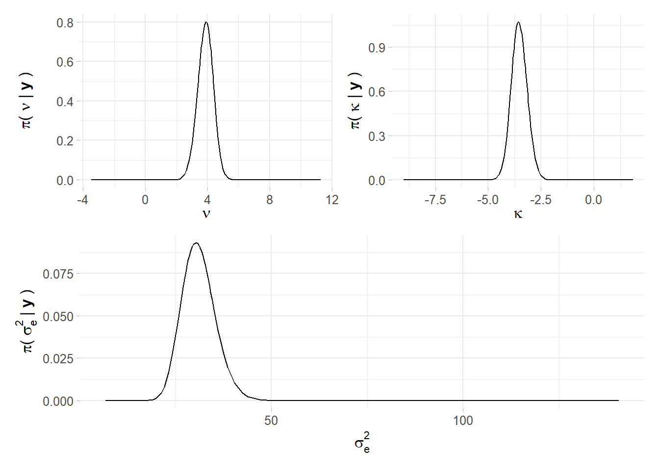
Figure 7.3: Marginal Hyper Parameter distributions for each element of Psi
7.5 Plot GMRF
Finally, it might be of interest to look at the latent field into the spatial field. The investigation can inform about possible omitted variables, i.e. how much variance the predictors are not able to capture in the response variable. From plot 7.4, for which it is chosen a grid of \(150 \times 150\) points, seems that the variance is correctly explained evidencing also three distinctive darker and relatively cheaper areas.
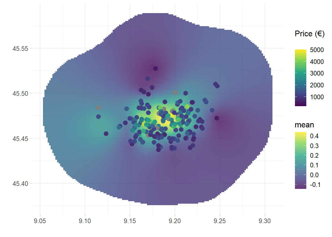
Figure 7.4: Gaussian Markov Random field of the final model projected onto the spatial field
7.6 Spatial Model Criticism
The model on the basis of the PIT 5.4.1 does not seems to show consistent residual trend nor failures (meaning bizarre values in relation to the others) i.e. $fails = $ 8 outliers. The fact that the distribution is seemingly Uniform 7.5 tells that the model is correctly specified. This is summarized by the LPML statistics which accounts for the negative log sum of each cross validate CPO, obtaining 6.681.
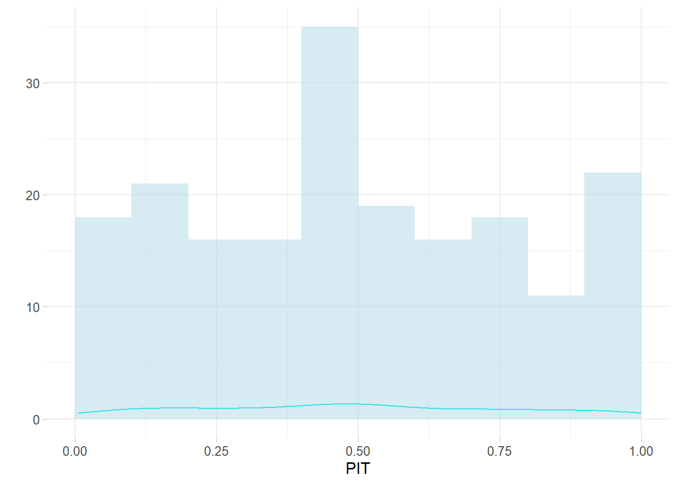
Figure 7.5: PIT cross validation statistics on \(model_final\)
7.7 Spatial Prediction on a Grid
A gridded object is required in order to project the posterior mean onto the domain space. Usually these operations are very computationally expensive since grid objects size can easily touch \(10^4\) to \(10^6\) points. For the purposes of spatial prediction, it is considered a grid of \(10km \times 10km\) with \(100 \times 100\) grid points. The intention is to chart the price smoothness given the prediction grid, alongside the corresponding uncertainty i.e. the standard error. Higher prices in 7.6 are observed nearby the points of interest in ??, however the north-ovest displays lower monthly prices. The variance is ostensibly considerable within the domain and unsurprisingly decreases where data is more dense.
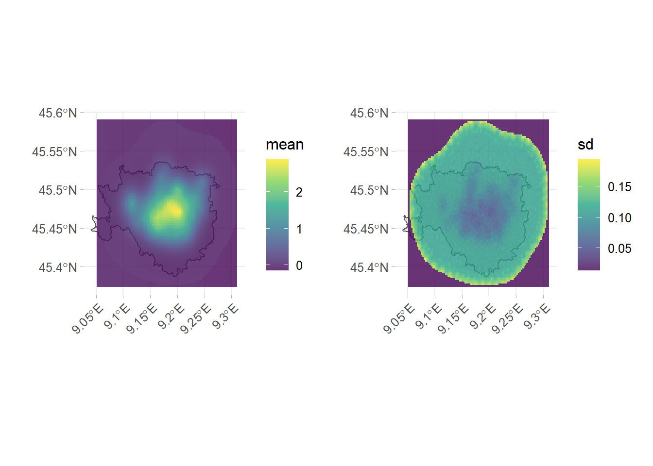
Figure 7.6: Prediction on predictive posterior mean a 122X122 grid overlapped with the Mesh3